I’m a big fan of AmiBroker, particularly the speed and flexibility it provides for backtesting trading strategies. However, one thing that is not particularly straightforward in AmiBroker is combining multiple strategies into a single system. Many quantitative (a.k.a. systematic) traders, myself included, use more than one strategy to help smooth their portfolio returns. The idea is that when one strategy is underperforming or is in a drawdown, other strategies can “pick up the slack” and minimize the pain. This works best when the individual strategy returns are not highly correlated.
If you’re trading your portfolio from a single brokerage account, then the most accurate way to model trading multiple strategies is to build all the logic into a single backtest. Before we can even start down that path, we would need to decide how the strategies would coexist in live trading. Some questions to consider include:
All of the issues above can handled via AmiBroker’s Custom Backtest (CBT) interface along with liberal use of static variables. However, it won’t be a trivial exercise.
Another approach, although imperfect, is to simply combine the equity curves of the two strategies. At a high level, this is quite straightforward:
The advantages of combining equity curves in this way are:
Of course, any shortcut will come with some disadvantages as well, including:
I recently built my own Equity Combo utility to combine two equity curves. Why only two at a time? Because rather than just combining one equity curve for Strategy A with one for Strategy B, I wanted to start by running optimizations on both strategies, saving an equity curve for each variation produced by the optimization run. My Equity Combo utility then allows me to examine all possible combinations of a Strategy A equity curve with a Strategy B equity curve, reporting the following metrics for each combination:
Notice that all my metrics can be determined from the individual and/or combined equity curves, without any knowledge of individual trades. You would surely have your own list of metrics that are of interest.
My utility also allows me to specify the percentage of equity allocated to A and B, as well as the rebalance frequency (Never, Daily, Weekly, Monthly, Quarterly, Annually). And finally, it can save each of the combined equity curves so that I can combine one or more of them with yet another base strategy (Strategy C) to find the total effect of adding new strategies to my portfolio.
The best part? The entire utility is only about 450 lines of AFL code, even with ample comments, blank lines for readability, etc. If you’re interested in learning more, please feel free to contact me.
Finally someone who gets it, past performance CAN be indicative of future returns!
For starters, what else is there? More importantly, the only thing that really could be indicative of future results is the demonstration of a repeatable process - and that would be reflected in the past performance revealed by the reliable back-test of a quantitative trading strategy.
I'm referring to a recent Bloomberg article titled 'A Manager's Past Performance Matters More than Ever', allow me to present you some excerpts - but please take a read for yourself.
The theory [that past performance is not indicative of future results] rests on some key assumptions, namely, that the money manager is a human whose basis or “investment philosophy” for decision making is discretionary, variable and opaque. But in today’s age of data and algorithms, the theory should be revisited. For starters, algorithms are driven by an explicit “objective function.” If the investment process is algorithmic and invariant then a track record demonstrating how the basis and the process performed under different regimes should provide an expectation of its performance in similar market regimes.
The author (Vasant Dhar) goes on to talk about a compelling track record (by Bernie Madoff!) and asks how we should interpret such a history.
Ostensibly, such a track record should matter. However, one obvious question is whether the length of the track record is sufficient to create an expectation of future performance. Equally important is whether the past record was produced by a repeatable, verifiable process reflecting an investment philosophy that will be followed in the future....
The first question is easier to answer. Analytically, the amount of data needed to determine statistical significance depends on the frequency of decisions. All else being equal, a higher-frequency program’s return distribution will have a lower variance than that of a lower frequency program due to shorter holding periods — it will make or lose less per decision. This lower variance and larger sample size of decisions over a specific period provides more information relative to a program with higher variance and fewer decisions.
On the Top Traders Unplugged podcast I've frequently heard Neils (the host) ask his guests whether they would prefer to evaluate a fund by looking at a track record, or a back test of the current strategy. It's not surprising to me how often they decide on the back test. Despite the fact that actual performance indicates a great deal (and I'm not taking away from that), that record could have come through various strategies at different times, using different decision-making processes (or even different individuals altogether) and thus it can be hard to take that information and extrapolate it into future expectations. However, taking a back test of the current strategy and getting an idea of how the exact system which is currently running, performed over various conditions in the past, tends to provide (me at least) more confidence in what it might do in the future. There are plenty of footnotes, exceptions, qualifiers and discussion that could properly be had on the subject, but even in simplifying, I can stand behind this message and wish it were told more often.
Managers, ideas and strategies will come and go, but good process gives a numbers guy like me confidence.
We frequently get asked about 'getting started in trading'. The truth is, it's a long journey, don't believe the hype (and certainly don't pay for any of it until you know what you're doing), but you do need to start somewhere and it's a big head-start if you can go directly to resources that represent genuine value. Start poking around the links here, make a start and see if you uncover a real passion. You're going to need that.

I think I'm with the 99% of other traders out there who can't help but mention the Market Wizards books first and foremost. Hearing individual's actual stories gives me the most food for thought (which is also why I love podcast interviews more than anything these days). The two simplest collections of great, up-to-date trading books on the market are easily found on the websites of two trading podcasts in fact. So simply take a look at the books suggested by all of the interviewees on these podcasts:
If you're really just getting started and you need to learn the basics of charting & technical analysis:
Then there are individual educators who are no-hype, thoughtful and practical, depending on your trading style (not focussed on systematic trading though). I'm including some "mindset" material here:
However, as I mentioned, I think the best way to begin, and then to keep learning and keep up to date, is to play trading and investing podcasts while you're at the gym, in the car, on your bike or at your desk! There's so much to learn here (so I'm just going to list a bunch!):
"Once you stop learning, you start dying"
Albert Einstein
Clearly there's a lot to choose from there, enjoy!
This is a placeholder for the next exciting blog I'd like to write on getting into the detail of building an algo.
My colleague Dave Di Marcantonio runs several web sites, including AmiBroker Courses where I sell some of my training courses. Dave recently published an introduction to trading automation, sometimes referred to as auto trading. Dave’s course also provides details about Alera Portfolio Manager, a new trading automation solution. APM can be integrated directly with AmiBroker but also works with other signal generating tools.
If you’re interested in automating your quantitative trading strategies, I encourage you to check out the course.
Trading or Investing Automation for AmiBroker Users made Simple
Recently I gave a presentation describing the process of creating and validating a simple trading strategy using AmiBroker. In this case, the instruments traded were the NIFTY and Bank NIFTY indices from the NSE in India, and the primary indicator used was the SuperTrend indicator. Although the performance results of the strategy are quite respectable, the real purpose was to introduce traders to the tools and methodologies that can be used to develop effective strategies of their own.
You can view the presentation linked above (my apologies for the less-than-stellar quality), or you can simply review the slide deck. As always, let me know if you have questions or comments. AFL used for the tests and an Excel workbook containing results are available upon request.
In a previous post we examined how back test results could be summarized for different market types. In today’s post, we’ll look at how we can use that information to tune our strategy for live trading.
As the basis for this exercise, we will use a modified version of the short mean reversion strategy known to Trading Markets customers as Bear Over-Reaction. While I cannot divulge all the specifics of this proprietary system, the basic rules are as follows:
A Setup occurs when:
Short the stock on the day following Setup using a limit order [2,4,6,8] % above the Setup close. Up to 5 open positions are allowed, with 20% of available equity allocated to each position.
When any of the following conditions occur on the close, Cover the position at the next open:
The values shown inside square brackets are the parameters that we will test during our AmiBroker optimization. Note that 3 x 2 x 4 x 2 x 3 gives us 144 unique parameter combinations or strategy variations.
To begin, we will test each of the 144 variations from 1/1/2000 through 12/31/2010. Summary results for the 10 variations with the highest Compound Annual Return (CAR) are shown in the table below.
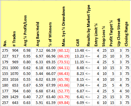
While the return numbers are not bad, the Max Drawdown (MDD) values are pretty scary. Not too many traders have the stomach to lose 60-70% of their trading capital. Even so, this gives us a place to start.
Now let’s jump ahead and see how these top performers did over the next 5+years, from January 1, 2001 through January 31, 2016:
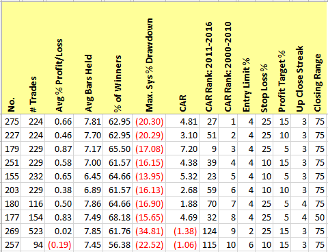
Uh oh! Here we see proof of the ever-popular warning “past performance is not a guarantee of future results”. Of the Top 10 variations for our initial 11-year test period, only one of those variations was still in the top ten over the next 5 years (variation 179). The new Top 10, shown below, uses different combinations of the parameter values:

The worst part is that we had no way to predict which variations would be the most successful following our initial testing. The best CAR was produced by the variation that ranked 19th over the previous test period! This is where looking at different market conditions or types can help.
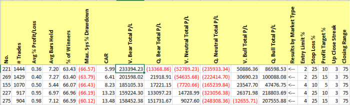
Going back to our results from 2000-2011, we will now add columns for each of six market types: Bear, Neutral, or Bull for market price action, and Quiet or Volatile for market volatility. For each market type, we have summarized the total dollars of Profit/Loss for trades whose Setup occurred when that market type was in effect.
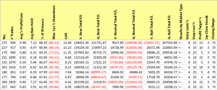
Notice that variation 275, which produced the highest overall CAR, also produced a decent amount of profit in Bear markets as well as Quiet Bull markets. However, it was more or less break even in Volatile Neutral markets, and lost lots of money in Quiet Neutral and Volatile Bull markets.
Instead of selecting one set of input parameters (i.e. one variation) to trade in all markets, what if we tried to use the best parameters for each market type. You could define “best” any number of ways, but for now we’ll stick with the very simple metric of total dollars of profit. If we re-sort our results to show the variations with the highest total P/L for V. Bear markets, we get:
In our strategy optimized for market type, on any day classified as Volatile Bear we would use an Up Close Streak of 3 days and a Closing Range of 75% for the Setup. We would then enter the trade on a 2% limit order, and use a stop loss of 25% and a profit target of 10%.
Repeating the process for the Quiet Bear market type, we see:

Therefore, on Quiet Bear days our Setup would also require an Up Close Streak of 3 days and a Closing Range of 75%, just like the Volatile Bear Setup. However, the limit entry would be 4% above the Setup close, and the stop loss would be at 25% and the profit target at 15%.
Repeating yet again for the Quiet Neutral market type, our results show:
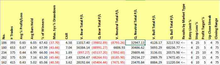
Now we can see that there are actually variations that have done well in this market type. On Quiet Neutral days, our Setup would be defined by a 4-day Up Close streak and a 75% Closing range. We would enter on a 6% limit order, with stops and targets of 25% and 5% respectively.
We continue this process for the remaining market types, and then combine the strategy parameters for each market type into one optimized strategy. Keep in mind that all of our strategy parameters were selected based on the back test results from 2000-2010.
So how does our optimized strategy perform from 2011 through January 2016?
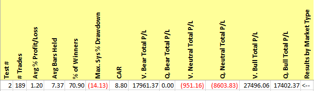
The Neutral market types still lost money. However, compare these results to Table 2, which showed how the former Top 10 from 2000-2010 performed from 2011 through January 2016. The optimized results shown in Table 8 had a higher CAR than any shown in Table 2, and had lower MDD than all but one of those variations. Best of all, we actually had a systematic way of selecting our strategy parameters.
In this example, we used a very simple method for defining the “best” results for each market type: the largest profit. We did not take into account drawdowns or any other factors that might be important to you when you trade. With additional thought and testing, it’s likely that we could improve on how to select the best variations for each market type. In addition, we would probably repeat the baselining process on a periodic basis rather than doing it just once and then using those “optimized” parameters for the next five years. Hopefully this article has given you some ideas on how to tune your own strategies for market conditions. As always, you can contact me if you need assistance.
One of the many interesting ideas put forth by Dr. Van K. Tharp is that you should not try to find a trading strategy that works in every type of market. Instead, he advises trading only those strategies that have performed well in the past under conditions similar to the current ones.
If you choose to adopt this approach to trading system development and selection, then the first step is to define a set of market types or conditions. One way to do this is to combine price action (bullish, neutral, bearish) with volatility (quiet, normal, volatile). For example, in today’s article I will use a six-month lookback on the S&P 500 index (SPX) to determine whether the market is bullish, neutral or bearish, and the CBOE Volatility Index (VIX) to determine whether the market is quiet or volatile (we won’t use “normal” as a volatility type here). The factors you choose to incorporate into your own market type definition will depend on your beliefs about the market and how you think those factors impact your trading results. Similarly, the timeframe over which you calculate your market type will be influenced by the type of trading you do. A day trader will likely have a very different way of defining the market type than a swing trader or momentum trader.
To illustrate the concept of reporting by market type, let’s consider a very simple mean reversion system based on the 2-period RSI, or RSI(2). The entry rules for long trades are:
And the exit condition is:
Both entry and exit will take place at the close of the day on which the signal occurs, and the back tests will cover the 10-year period from 1/1/2006 through 12/31/2015.
The table below shows a few key metrics for each of the 12 strategy variations: 4 RSI(2) entry values combined with 3 RSI(2) exit values. This was an “all trades” test, meaning that we took every available entry signal without regard to portfolio considerations like position sizing or capital constraints. The only restriction was that only one open trade per symbol was allowed at any given time.

We can see that the percentage of profitable trades (% of Winners) was very close to 69% for every variation. Therefore, let’s focus on the average gain per trade. The table entries are sorted from highest to lowest Avg % P/L, with the best performing variation (No. 21) producing a 0.83% gain by entering trades on an RSI(2) value below 5 and exiting when RSI(2) moves above 80. As we move across the top row from left to right, we see that variation 21 did not perform equally in all market types. In Bear and Neutral markets, the gain per trade was usually around 1.0%, but in Bull markets the gain fell to 0.44% when the market was Volatile and 0.79% when the Bull market was Quiet. So, if variation 21 was the only one we were trading, we might choose not to trade in Bull market types.
Now let’s focus on the column for each market type. In each of these six columns, the highest Avg % P/L is highlighted green. For the Volatile Bear market type, the highest Avg % P/L was produced by the same variation (21) that generated the best overall Avg % P/L. However, for the Quiet Bear market type, variation 24 produced a superior gain per trade of 1.62%. Although this is a simplified example which focuses on only one metric, it’s clear that we can extend this concept to help us to determine when to trade our base strategy, when to tweak our rule parameters, and when to consider sitting out altogether.
If we reverse the long rules to create a short system, we observe even more differentiation between the market types. On an overall basis, none of these variations comes out much above break even, despite the fact that the test did not account for commissions. However, the two Bear market types each identified some interesting variations of the strategy, while both Neutral market types and the Quiet Bull type would clearly not be worth trading as the strategy is currently written.

Please feel free to contact me if you’d like a copy of the Excel spreadsheet or if you need assistance adding this type of reporting to your AmiBroker back tests and optimizations.
Last night I revisited the topic of creating adaptive strategies for an audience from the AmiBroker Canada User Group and a local chapter of the Canadian Society of Technical Analysts. The presentation was well-received, and the audience asked thoughtful questions at the end. If you want to listen in, the recording can be found here.
I recently completed a client project that utilizes the SuperTrend indicator. The indicator is basically a variation on other types of volatility bands, using a multiple of ATR to define bands above and below the current average price. The SuperTrend line follows the lower band when the price is in an up trend (has most recently broken the upper band), and follows the upper band when the price is in a down trend (has most recently broken the lower band).
I have not used the indicator enough to have a strong opinion on its usefulness, although it seems to be particularly popular with traders from India. However, I had a hard time finding written definitions of the indicator, and the one that I did find was incorrect. I finally resorted to creating a definition by reverse engineering some code written by Rajandran R at www.marketcalls.in. I then wrote my own version in AmiBroker AFL in a way that makes it easy to use on a chart or in an exploration. In addition, the SuperTrend function could be easily copied to another AFL used for back testing or other AmiBroker analysis.
Here is the definition of the SuperTrend indicator that I derived from Rajandran’s code:
SuperTrend requires two parameters:
We begin by calculating preliminary values for the upper and lower bands as follows:
UpperBand = (High + Low) / 2 + (width * ATR(lenATR))
LowerBand = (High + Low) / 2 - (width * ATR(lenATR))
Next we examine the bands and the Close of each bar in the series to determine the trend:
If Current Close > Previous UpperBand Then Trend is UP
Else If Current Close < Previous LowerBand Then Trend is DOWN
Else Trend is unchanged from previous bar
The direction of the trend allows us to modify the preliminary band values, and also determine whether the SuperTrend line is currently following the upper or lower band:
If UP trend Then
    Current LowerBand = max(Current LowerBand , Previous LowerBand )
    Current Supertrend = Current LowerBand
If DOWN trend Then
    Current UpperBand = min(Current UpperBand , Previous UpperBand )
    Current Supertrend = Current UpperBand
Here is the AmiBroker AFL for the SuperTrend indicator:
/////////////////////////////////////////////////////////////////////////////
// Supertrend Indicator
//
// AmiBroker implementation by Matt Radtke, www.quantforhire.com
//
// History
// v1: Initial Implementation
/////////////////////////////////////////////////////////////////////////////

function SuperTrend(lenATR, width)
{
    nATR = ATR(lenATR);
    pAvg = (H+L) / 2;

    upperBand = pAvg + width * nATR;
    lowerBand = pAvg - width * nATR;
    isUpTrend = True;
    dn = DateNum();

    for (i=lenATR; i<BarCount; ++i)
    {
        if (C[i] > upperBand[i-1])
            isUpTrend[i] = True;
        else if (C[i] < lowerBand[i-1])
            isUpTrend[i] = False;
        else
            isUpTrend[i] = isUpTrend[i-1];

        if (isUpTrend[i])
            lowerBand[i] = Max(lowerBand[i], lowerBand[i-1]);
        else
            upperBand[i] = Min(upperBand[i], upperBand[i-1]);
    }

    super = IIf(isUpTrend, lowerBand, upperBand);
    return super;
}

lengthATR = Param("ATR Length", 10, 1, 100, 1);
widthBands = Param("Band Width", 3, 1, 20, 0.1);
st = Supertrend(lengthATR,widthBands);

Plot(st, "Supertrend("+lengthATR+","+widthBands+")", ParamColor( "Color", colorCycle ), ParamStyle("Style") );

Filter = True;
AddColumn(O,"Open");
AddColumn(H,"High");
AddColumn(L,"Low");
AddColumn(C,"Close");
AddColumn((H+L)/2,"Avg");
AddColumn(ATR(lengthATR), "ATR("+lengthATR+")");
AddColumn(st, "Supertrend("+lengthATR+","+widthBands+")");
DISCLAIMER – READ FULL DISCLAIMER HERE


